Container Based Reproducible Analysis for SLURM
17 Nov 2016You have a Python script. Actually, maybe you have a few, because you wrote a file with supporting functions, and you are happily churning away on your local machine. You then have a terrible, awful epiphany, and it looks something like this:
So I just need to run this on 500 datasets…
This issue is relevant to scaling. You need a cluster environment to run your code a gazilion times.
Let me calculate how much memory that I need for this. Oh #$@#.
This is another use case where we need a cluster environment, but just to get a crapton more memory than our little ‘puter can afford.
I need to send this to my colleague… how and what did I install again?
This final issue on your hands is one of reproducibility. You have been happily going along, installing stuff (whatever, it works). But, then your colleague on the East Coast tries to run something, and “Hey, this doesn’t work.”
But it works fine for me!
/facepalm Let’s avoid the above entirely by building a container-based, SLURM ready thing. Are you ready? If you are just interested in the container part, I recommend skipping the first sections and going straight to putting the application into containers. Otherwise, here are the steps we are going to be covering today:
Quantum State Diffusion: an example application
Our example application comes by way of a Physics graduate student at Stanford. He both needed to scale, and had a collaborator that missed installation of a particular dependencyu. If you are interested, you can look at the original state of his code base here, and the final thing is here. There was one Python script with hardcoded variables to run a simulation (this one), and a second with a saving function (this one). If you look at the README.md in the repo, you’ll notice that he mentions several special packages that need to be installed, including a standard package with custom changes. I took a look at this repo, and first (in my head) outlined a set of general things I wanted to do:
- Make sure we have version control set up (Github, already done)
- Make an account on Docker Hub to build our container automatically
- Wrap the main calling functions into an executable script
- (Optionally) organize supplementary files and packages
- Put the application into containers
- Write a SLURM submission script (and docs)
In a nutshell, we are going to wrap all code and dependencies into a container, and then run the container on a SLURM cluster. He’s also going to be able to provide the container based environments for his collaborators to use and (further develop together).
0. Version Control with Github
If you want to collaborate on code, have a complete record of your changes, have a nice way to work on different branches, you need to make an account on Github, and this means having Git installed. Talking about version control is outside of the scope of this post, but if you have questions, please reach out.
1. Build Containers with Docker Hub
Importantly, we are going to be using Docker Hub to connect to our Github repos and automatically build Docker images whenever we push. Signing up is a simple process, and you will want to immediately hook up the repo where you are storing your code. This is called an automated build and it’s a little bit hidden in the interface. You want to click Create –> Create Automated Build:
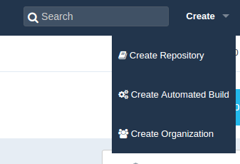
You then have the choice to select from Github or Bitbucket.
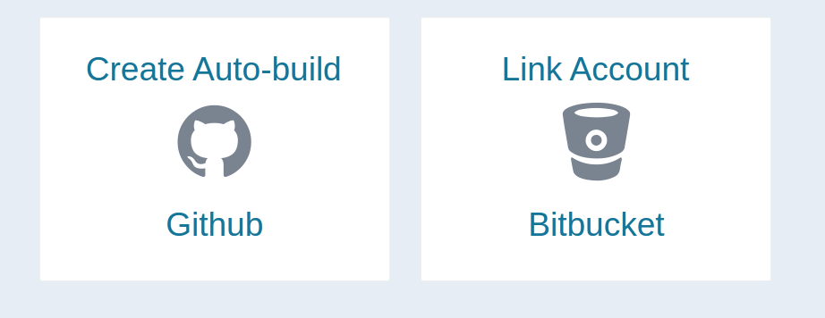
You are required to enter a description, and then click Create. By default, your builds will be built on pushes to the master branch. If you want to alter this behavior, you should click "Click here to customize this behavior". This default setup should meet our need. We are now set up on Docker Hub, let’s go back to the code!
2. Wrap the main calling functions into an executable script
Both a Docker and a Singularity container have an ability to execute something when you run them like scripts. This means that, if you have a function:
def print_hello_world(name="Schloopy",screen_print=True):
    response = "Hello World, and %s" %(name)
    if screen_print == True:
        print(response)
    return response
which we would run like this from within a Python interpreter:
In [2]: print_hello_world()
Hello World, and Schloopy
Out[2]: 'Hello World, and Schloopy'
You need to be able to run this directly from a command line (outside of a Python terminal or notebook) something like this:
helloworld --name Schloopy
Hello World, and Schloopy
You need a basic script that understands input arguments, and what to do with them. I’ve made a simple template that can help with this:
PROTIP: If you want this script to be an executable installed to the user’s bin when pip installs the package, you should reference it in the
setup.pyas aconsole_scriptsobject inentry_points:
 entry_points = {
        'console_scripts': [
            'helloworld=helloworld.scripts:main',
        ],
    },
If you are interested, let’s talk in more detail about the parts of this script. If not, feel free to copy paste, edit, and move on to the next section.
The executable at the top
The top of the script looks like this
#!/usr/bin/env python
This command is telling the computer what interpreter to use. In this case, we are directing it to use the running Python environment (found first in the $PATH).
The comments sections
You should start to get comfortable with writing lots of comments and notes about your functions, with your functions. Why? Because these comments will seamlessly transform into documentation (see Sphinx), and trust me, you are going to need it when you come back in a few months and have forgotten how your code works. For the header, you should minimally have the name, a brief description, and perhaps the author and any license information. For each function, you should have something like this:
def print_hello_world(name="Schloopy", screen_print=True):
    '''print_hello_world will print "Hello World" followed by a name
    :param name: the name to print, str. Default: "Schloopy"
    :param screen_print: boolean, if True (default), prints
    :returns: response, str, the full string response
    '''
    response = "Hello World, and %s" %(name)
    if screen_print == True:
        print(response)
    return response
Generally, every function should have comments, even if they are minimal. It makes your code look really nice, too :)
The Parser
Each language has it’s own “easy” way to take in input arguments (and likely I will provide templates or examples for different languages), but for now we will focus on Python. Python has the module argparse that makes it really easy to turn a set of Python scripts into an executable. I like to have a small function that makes the parser, and then returns it:
def get_parser():
    '''get_parser returns the arg parse object, for use by an external application (and this script)
    '''
    parser = argparse.ArgumentParser(

    description="This is a description of your tool's functionality.")

    # String
    parser.add_argument("--string",
                        dest='string',
                        help="string argument with default None",
                        type=str,
                        default=None)

    # Integer
    parser.add_argument("--integer",
                        dest='integer',
                        help="integer argument with default 9999",
                        type=int,
                        default=9999)

    # Boolean
    parser.add_argument('--boolean',
                        dest='boolean',
                        help="boolean argument when set, returns True",
                        default=False,
                        action='store_true')
    return parser
Look at the docs for more advanced usage. The general thing you are going to do is use the function add_argument, and let’s look at an example from our Physics script to see what that might look like:
    # Seed
    parser.add_argument("--seed",
                        dest='seed',
                        help="Seed to set for the simulation.",
                        type=int,
                        default=1)
- The first thing,
--seedis the argument that is going to be specified on the command line. dest: is the destination of the argument. For example, if the ArgumentParser is calledargs, our--seedargument is going to be found inargs.seed.help: is a nice message to print to the user in the command line usage. One of the jobs of argparse is to make sure everything required is provided, and if it isn’t, it is going to spit out this helper section. This means that you should be detailed about your variables here.type: is the type of variable, a python class (eg,str,int,float) that the variable is expected to be.default: gives the variable a default value, if the user did not set it.
After we create a parser, we are going to put the following in our main() in order to use it:
def main():
    parser = get_parser()
    try:
        args = parser.parse_args()
    except:
        sys.exit(0)
The function get_parser() that we defined above is going to return an argparse.ArgumentParser, the variable args, that we are going to find all of our arguments in. We can then move forward in our executable script to run particular functions that we’ve imported depending on what inputs the user has provided. An important thing to review, since it is slightly different from the standard int or str types, is talking about how to deal with booleans. For example, let’s say that I want to use my print_hello_world function in some pipeline that, for reasons unbeknownst to me, actually printing something will explode the machine. I might want to create a flag --silent that when I run my script, will prevent the print, something like this:
helloworld --name Schloopy --silent
How would that look for the argument parser? Something along the lines of this:
    parser.add_argument("--silent",
                        dest='silent',
                        action="store_true",
                        help="Suppress all printed output",
                        default=False)
I would then pipe the variable into my hello world function call like this. To be ridiculously clear about the variables, I’ve written this in more detail than necessary:
silent = args.silent

if silent == True:
    # If flag present, don't print to the screen
    screen_print = False
else:
    # If flag absent, use the default and print!
    screen_print = True

response = print_hello_world(screen_print=args.silent)
Generally, think of the default as what will happen when there is no flag. When you see action think of this as the parser telling you
“This is what I’m going to do if I see that flag. If the user tells me
--silent, I’m going to store the variable as True.”
You can take a look at the Physics example to see a real use case that covers a few of these examples across a large array of arguments.
The Main Function
It’s a nice, and simple standard in most languages to have some way of specifying a “main” function. In Python, there is a way for a script to know if you are calling it. If we look at the bottom we see:
if __name__ == '__main__':
    main()
In layman’s terms, this snippet says “If someone is executing me, do whatever I tell you in this statement. In this case, we are just running the function main(). Now you can scroll up, and see that the body of the code is in this function, including the bit to get the parser. The level of detail in this section is up to you. If you have a simple or isolated thing you are writing this for, you might just write the bulk of your code in this main, and perhaps import some supplementary functions from modules or other included Python files. However if you have a more complex set of functions, or want this executable to be able to perform different things at different times, I would suggest the following approach:
- Write a proper Python package.
- Import the various important functions into your executable
- Link the function imports to command line arguments, making sure that the user has provided the data you need for each one.
In this scenario, your executable script isn’t doing the heavy lifting, it’s just re-routing the user to the function that the user wants, and making sure the inputs are provided and correct.
Saving stuff
How should we save things? There are two important things to talk about - data structures, and user control.
Data Structures
What is the output that your function(s) are intended to produce? First, this needs to be well organized, and fit to a standard as best as you can. For Python, my data structure of choice is a pickle, because let’s be real, anything that I can dump and load on demand is pretty excellent. Pickle is a nice format because it optimizes read and write performance, and compressing your results. However, the drawbacks of Pickle are that if someone found a Pickle file on a computer somewhere, without a Python interpreter they can’t really peek inside. For smaller data, or a data output that is table friendly and can be read in by other analysis software more easily, saving to comma separated or tab separated (.tsv, .csv) is a good idea. The saving format, again, is up to you, and whatever strategy you choose, keep in mind how the data is intended to be stored and used.
What to save?
What I like to do is save data, whether that be a bunch of lists, numbers, or arrays and data frames, to a nice dictionary (the values are the objects), with keys corresponding to a standard label or descriptor to tell what it is. If you are doing a computational analysis of any kind, you should make it a standard practice to save your analysis parameters to this object. For example, here we are putting the arguments from the parser into variables and a dictionary simeotaneously:
    # Set up commands from parser
    params = dict()
    ntraj = params['Ntraj'] = args.ntraj
    seed = params['seed'] = args.seed
    duration = params['duration'] = args.duration
    delta_t = params['delta_t'] = args.deltat
    Nfock_a = params['Nfock_a'] = args.nfocka
    Nfock_j = params['Nfock_j'] = args.nfockj
    downsample = params['downsample'] = args.downsample
and then our saving function in utils.py always has an optional params argument that will update a dictionary with parameters:
def save2pkl(data,file_name,obs, params=None):
    ''' save2pkl saves to a pickle file
    :param data: the data dictionary object
    :param file_name: the file name (with extension) to save to
    :param obs:
    :param params: extra params to add to the save object
    '''
    logging.info("Saving result to %s.pkl", file_name)
    mdict = prepare_save(data,file_name,obs,params)
    output = open("%s.pkl" %file_name, 'wb')
    pickle.dump(mdict,output,protocol=0)
    output.close()
    logging.info("Data saved to pickle file %s", file_name)
You would of course want to be sure that there are no parameter names (they keys in the params dictionary) that would overwrite data in your output data dictionary (data).
Naming Schemes
While it’s pretty standard to give the user control about where to save something, it’s not always clear how much should be given to name output. In our Physics example, I decided that I wanted to capture the simulation parameters in the output file, including the regime, and other input arguments. Thus, I gave the user control to specify an output folder (if not specified it generates a path to the present working directory) and then handled the file naming as follows:
    ## Names of files and output
    Regime = "absorptive_bistable"
    param_str = "%s-%s-%s-%s-%s-%s" %(seed,ntraj,delta_t,Nfock_a,Nfock_j,duration)
    outdir = ""
    if args.outdir != None:
        outdir = args.outdir
    file_name = '%s/QSD_%s_%s' %(outdir,Regime,param_str)
It’s also important to note that the default behavior I chose is to not save anything. You generally don’t want to be writing anything anywhere without the user asking for it. This of course depends upon your use case.
User Control
You should always make the saving of data, or not, very highly controllable by the user. This means giving the option to specify and output directory, and even specify different kinds of output or disable it all together (and perhaps just print to the screen for testing).
Logging
Every language has it’s own way to print stuff to standard streams. Python makes this ridiculously easy. You basically import the logging module, set up a default logger in your executable, and then and child processes (e.g., functions) called by your script will find the same logger configuration. Here is the simplest example I can come up with:
import logging

# Log everything to stdout
logging.basicConfig(stream=sys.stdout,level=logging.DEBUG)

# And then in main, or elsewhere...
logging.error("This is an error! Meep!")

pancake_status = "delicious"
logging.info("The pancake status is", pancake_status)
Check out more details in the module’s documentation. Logging is great for more sophisticated applications because it gives you control to send logs somewhere else (eg, a file), and allow a user to specify levels (e.g., have a debug mode).
Overview
By this point, we’ve done the following:
- Written our Python script into a main executable
- Handled input arguments to some degree
- Made it possible to save stuff, and allow the user to specify how this is done.
3. Organize supplementary files and packages
You could imagine doing all of the above, but instead of having files local in your repository, work by way of an official Python package that you’ve developed. If you choose to not create a package, and just want to keep a few simple files, here are some things to think about:
- Organize functions in supplementary files (modules) that are named logically. For example, functions to save and load files, or format things, I would likely want in something called
utils.py. A Class object might be in a file that mirrors the name of the class. Machine Learning or analysis functions might be in a file calledanalysis.py. It’s really up to you, but think about if someone else were to look at your code, and if they were looking for something in particular, would it be intuitively found? - Don’t be afraid to use folders to organize data and supplementary files. If you have an entire set of
.csvfiles that are inputs in the base directory, this might make it hard for the user or another developer to find other things. Make a folder calleddataorinputs, or even better, something more descriptive.
The next thing we want to do is put this application into containers. We are going to use Docker and Singularity.
4. Put the application into containers
We’ve gone through a lot, and we are just getting to the fun part! This is where we want to write different “build files” that will produce containers optimized for our different use cases. Specifically, we are going to empower our user to run the Physics simulation in the following environments:
- Docker
- Singularity
- Local Environment
- Cluster (SLURM example)
Depending on your familiarity with containers, the first two are recommended to handle software dependencies. The third is “proceed at your own risk.” The last is basically wrapping the second (Singularity) to run in a cluster environment, because our other container, Docker doesn’t really work there.
Docker
For this container you need to install Docker. Let’s first look at what using our Docker image would be like. A Dockerized development environment means that, from our local machine, we can run the simulation with a Docker image.
docker run vanessa/quantum_state_diffusion --help
will show you the following (after a message about the font cache):
usage: make_quantum_trajectory.py [-h] [--seed SEED] [--ntraj NTRAJ]
	                          [--duration DURATION] [--delta_t DELTAT]
	                          [--Nfock_a NFOCKA] [--Nfock_j NFOCKJ]
	                          [--downsample DOWNSAMPLE] [--quiet]
	                          [--output_dir OUTDIR] [--save2pkl]
	                          [--save2mat]

generating trajectories using quantum state diffusion

optional arguments:
  -h, --help            show this help message and exit
  --seed SEED           Seed to set for the simulation.
  --ntraj NTRAJ         number of trajectories, should be kept at 1 if run via
	                slurm
  --duration DURATION   Duration in ()
  --delta_t DELTAT      Parameter delta_t
  --Nfock_a NFOCKA      Parameter N_focka
  --Nfock_j NFOCKJ      Parameter N_fockj
  --downsample DOWNSAMPLE
	                How much to downsample results
  --quiet               Turn off logging (debug and info)
  --output_dir OUTDIR   Output folder. If not defined, will use PWD.
  --save2pkl            Save pickle file to --output_dir
  --save2mat            Save .mat file to --output_dir
What just happened? When we do Docker run, it first looks for a set of layers (compressed tarballs that are put together like Legos to form an entire image) required for the image. If we have them, great! It puts them together, and runs this virtual machine container thing (let’s leave it at that level of detail for now) on our computer. If we don’t have them, it looks for them and downloads them from the Docker Registry and then runs the container. Remember that Docker Hub account we made earlier? That’s the place in the cloud place where your image lives. Then you must be curious, how do we create a Docker image? We create a specification, called a Dockerfile, for it.
The Dockerfile
The Dockerfile is the specification that the command line tool docker knows how to build images from. Yes, this means that you can have these things laying all over your computer and build images without having to connect to Docker Hub. This is also a simple, and easy format to understand. You can look at the full Dockerfile for the Physics container, or the walked through version here:
FROM: the FROM statement is a way of bootstrapping another image, which means not starting from nothing, and first dumping in whatever layers are defined in that image. In the example below, we use ubuntu 16.04, and take a look, it has it’s own Dockerfile!. How nice that we don’t have to redo all that stuff, we can capture it with one line.MAINTAINER: is a piece of metadata where you would expect to find the right person to contact about the image. I usually put my email address and/or nameENV: This is a way to define an environmental variable. In the example below, I am setting the variablePYTHONBUFFEREDto1.RUN: Is the command you are going to be using most often. It’s how you run things! Given the amount of Python things that I do, I use it most often to install system packages withapt-get, and then download things withgitorwget, and then install Python packages withpip.WORKDIR: sets the working directory. If you do a “cd” it will work for commands on the same line, but the working directory on the next line is going to be the root again. This is why you need this argument.ADD: There is a fine distinction between ADD and COPY, and likely I’ll get it wrong here. As far as I can tell, both ADD and COPY can be used to move files from your local machine into the container. This works for all files in a folder (if you specify the folder as the source) or a single file. The difference I think has to do with what is allowed for the source, eg:
ADD <src> <dest>
If you use ADD, the <src> can be a URL, or you can give it a compressed archive, and it will unpack it for you. For details about all of the above and examples, see the official docs. Now, let’s take a look at the general format that I would follow for your file. For our example, we are going to follow the general structure:
- Imports and metadata (Maintainer, From, yadda yadda)
- Environment variables
- Installation of OS specific software
- Make directories / file structure
- Install dependencies
- Move stuff into your container
- Clean up
- Define what happens when you run it.
Here is how that might look:
FROM ubuntu:16.04
MAINTAINER "vsochat@stanford.edu"

# SET ENVIRONMENT VARIABLES HERE
ENV PYTHONUNBUFFERED 1

# INSTALL OS SPECIFIC STUFF HERE (apt-get, yum etc)
RUN apt-get update && apt-get install -y \
    libopenblas-dev \
    gfortran \
    libhdf5-dev \
    libgeos-dev \
    build-essential \
    openssl \
    wget \
    git \
    vim

# MAKE DIRECTORIES HERE
RUN mkdir /data

# INSTALL DEPENDENCIES HERE

# Install anaconda 3
RUN wget https://repo.continuum.io/archive/Anaconda3-4.2.0-Linux-x86_64.sh
RUN bash Anaconda3-4.2.0-Linux-x86_64.sh -b -p /usr/local/anaconda3
RUN export PATH=/usr/local/anaconda3/bin:$PATH
RUN echo "export PATH=/usr/local/anaconda3/bin:$PATH" >> $HOME/.bashrc
RUN /usr/local/anaconda3/bin/conda install -y pyqt

# Install modified sdeint package
RUN git clone https://github.com/tabakg/sdeint
RUN cd sdeint && /usr/local/anaconda3/bin/python setup.py install


# MOVE STUFF FROM YOUR MACHINE INTO THE CONTAINER HERE

# Add code to container
RUN mkdir /code
WORKDIR /code
ADD requirements.txt /code/
RUN /usr/local/anaconda3/bin/pip install -r /code/requirements.txt
RUN apt-get remove -y gfortran
ADD . /code/

# CLEAN UP
RUN apt-get autoremove -y
RUN apt-get clean
RUN rm -rf /var/lib/apt/lists/* /tmp/* /var/tmp/*

# DEFINE HOW IT RUNS
ENTRYPOINT ["/usr/local/anaconda3/bin/python","/code/make_quantum_trajectory.py"]
Some random good practice points:
- Try to chain commands as needed. For example, if you need to cd into a folder, you want to do something along the lines of
cd installfolder && python setup.py installbecause if you put it on two separate lines, you are going to get an error that the script wasn’t found. If you need to change a directory and stay there, useWORKDIR. - For Python, it’s really nice and easy to install things using a
requirements.txtfile. - You should remove extra stuff that isn’t needed at the end (see
CLEAN UP) - Yes, you can still include comments with
#in the Dockerfile. - The entrypoint should have different commands in a list style thing (see above). It should also point to very specific executable files, in the case that you have multiple.
How does the container map to my machine?
Let’s go back to our Physics example. We are going to want to save data, and given that the container runs and goes away, if it isn’t saved somewhere on our local machine, it’s pretty much useless to run in the first place. This is why we created this /data folder inside the container, remember this?:
# MAKE DIRECTORIES HERE
RUN mkdir /data
This is incredibly powerful, because we are going to tell the executable to save data to this location inside the container, but then we are going to map that location to somewhere on our local machine. Docker has the -v argument for this exact purpose. It means “volume” and follows the standard:
-v <local>:<container>
For our application, we will first specify the output directory to the /data folder in the container using the --output_dir argument, and then we will map some directory on my local machine to this /data folder:
docker run -v /home/vanessa/Desktop:/data \
             vanessa/quantum_state_diffusion --output_dir /data --save2pkl
The above will produce the following output:
	INFO:root:Parameter Ntraj set to 1
	INFO:root:Parameter Nfock_j set to 2
	INFO:root:Parameter duration set to 10
	INFO:root:Parameter delta_t set to 0.002
	INFO:root:Parameter downsample set to 100
	INFO:root:Parameter Nfock_a set to 50
	INFO:root:Parameter seed set to 1
	INFO:root:Downsample set to 100
	INFO:root:Regime is set to absorptive_bistable
	Run time:   2.1634318828582764  seconds.
	INFO:root:Saving pickle file...
	INFO:root:Saving result to /data/QSD_absorptive_bistable_1-1-0.002-50-2-10.pkl
	INFO:root:Data saved to pickle file /data/QSD_absorptive_bistable_1-1-0.002-50-2-10
The final output will be in the mapped folder - in the example above, this would be my Desktop at /home/vanessa/Desktop/QSD_absorptive_bistable*.pkl
How do I get inside the container?
If we run the above, we get a thing output, and the container goes away. What if we want to work from inside the container? We can! You may want to inspect the data using the same environment it was generated from, in which case you would want to shell into the container. To do this, you can run:
docker run -it --entrypoint=/bin/bash vanessa/quantum_state_diffusion
The it means “interactive terminal.” Do you remember the ENTRYPOINT that we defined in the Dockerfile?
# DEFINE HOW IT RUNS
ENTRYPOINT ["/usr/local/anaconda3/bin/python","/code/make_quantum_trajectory.py"]
The command above says
“just kidding, please run me a bash shell instead!”.
Then we are taking inside the container (cue Twilight Zone music). If you type ls you will see that we are sitting in the /code directory that contains the core python files, and this is because this was the last call to set the WORKDIR in our Dockerfile. This means that we can run the analysis equivalently:
	/code# python make_quantum_trajectory.py --output_dir /data --save2pkl
	INFO:root:Parameter downsample set to 100
	INFO:root:Parameter duration set to 10
	INFO:root:Parameter seed set to 1
	INFO:root:Parameter Nfock_j set to 2
	INFO:root:Parameter Nfock_a set to 50
	INFO:root:Parameter delta_t set to 0.002
	INFO:root:Parameter Ntraj set to 1
	INFO:root:Downsample set to 100
	INFO:root:Regime is set to absorptive_bistable
	Run time:   2.183995485305786  seconds.
	INFO:root:Saving pickle file...
	INFO:root:Saving result to /data/QSD_absorptive_bistable_1-1-0.002-50-2-10.pkl
	INFO:root:Data saved to pickle file /data/QSD_absorptive_bistable_1-1-0.002-50-2-10
and the data is inside the container with us! Great.
	root@4420ae9e385d:/code# ls /data
	QSD_absorptive_bistable_1-1-0.002-50-2-10.pkl
How can my collaborators customize the image?
Let’s say you do the above, you have the Docker image building on Docker Hub (and thus available to anyone that runs the commands above), and now you have a collaborator that says:
Hey, dawg. This dimensionalty reduction function that you used? I want to try something a little different.
And you really want to respond:
Different, bruh?! There is only one way, the right way, and that’s the way I did it.
No no, don’t say that! Support his or her effort to collaborate on your code. You technically could ask them to make a PR to a different branch, or make them a collaborator to do whatever they want with your code, but that’s kind of annoying and hard. What you’d really like them to be able to do is just make some changes locally, and then test them. This is the perfect use case for building a Docker image locally. Another good use case is if you have some code and a Dockerfile that you (for some reason) don’t want to put on Github or Docker Hub. You can build the image by doing the following:
      git clone https://www.github.com/researchapps/quantum_state_diffusion
      cd quantum_state_diffusion
      docker build -t vanessa/quantum_state_diffusion .
Note the . at the end of the command to specify the present working directory. Don’t forget it!
And then the layers are on your machine, and you can use the image as we did before. Note that when you are developing your image, any changes that you make to the Dockerfile you will need to rebuild. Luckily, Docker is smart about this, and each line maps to one of those “layer” things. If you make a change, only the layers that are changed will need to be re-build (which hopefully isn’t the entire thing).
Singularity
Docker is amazing for development locally, for small reproducible products, and mostly anything in the cloud. But if you are a researcher wanting to run a container in a cluster (HPC) environment, it’s likely not going to be installed. Singularity is a container that is HPC friendly, meaning that it can be run on a cluster environment. The container itself, a file that sits on your computer, can be dropped into a folder on your cluster, and run like a script! For our example, we are going to provide the user with a Singularity file that, akin to the Dockerfile, Singularity knows how to build an image from. Actually, we are going to cheat a bit. Until Singularity has its own Docker Hub equivalent (it’s under development), we are going to bootstrap the Docker image that we just created! Pretty cool :)
Install Singularity
Instructions can be found on the singularity site.
The Singularity File
Guess how much we get to cheat? A lot! We are basically going to tell Singularity to dump the guts of the Docker image we just created into a Singularity one (diabolical laugh). To do this, we create a Singularity file in our repository:
Bootstrap: docker
From: vanessa/quantum_state_diffusion

%runscript

    exec /usr/local/anaconda3/bin/python /code/make_quantum_trajectory.py "$@"


% post

    mkdir -p /share/PI
    mkdir -p /scratch
    mkdir -p /local-scratch
    sudo chmod -R 777 /data
    echo "To run, ./qsd.img --help"
This file is super simple, at the top we have the following:
Bootstrap: tells Singularity what kind of OS/thing we are bootstrapping. In this case, we are just smiling and pointing to Docker.From:is akin to the Docker From, it specifies the image that we are going to use. In our case, it’s the one we just made!%runscript: This section has the commands that the container is going to execute when you run it as an executable. You will see this looks pretty similar to what we had in our Dockerfile, except we add this weird looking"$@"at the end. This will capture all other input arguments from the user. We also add anexec, which I believe hands the container process to that command.%post: This is the section where we would install stuff, or any other post Bootstrap commands. It’s run once after bootstrap, and that’s it. What I like to do is add a line or two of quick documentation for the user (eg, look at the--help) and I’ve also added commands to create directories that are going to mapped on the sherlock (slurm) cluster.
That’s it! Now let’s use Singularity to create and bootstrap the image!
Bootstrap the image
Bootstrapping (as of version 2.2) means creating an image, and then pointing it at the build file, Singularity:
    sudo singularity create --size 4000 qsd.img
    sudo singularity bootstrap qsd.img Singularity
You will notice that I specified a --size when I created the image, and this is because the default size is too small for the stuff I’m dumping into it. If I don’t specify this size, it’s going to give me an error about disk space. Bootstrapping looks like this:
sudo singularity create --size 4000 qsd.img
Creating a new image with a maximum size of 4000MiB...
Executing image create helper
sudo Formatting image with ext3 file system
singularity bootstrap Done.

sudo singularity bootstrap qsd.img Singularity
Bootstrap initialization
Checking bootstrap definition
Executing Prebootstrap module
Executing Bootstrap 'docker' module
From: tabakg/quantum_state_diffusion
IncludeCmd: yes
tabakg/quantum_state_diffusion:latest
Cache folder set to /root/.singularity/docker
Downloading layer: sha256:2e6f0c61a2d84d4345db0b1be47cb64fc8346f55a10cebde915901b9716330da
Downloading layer: sha256:3a98e44275526690ab18461998ca97106b93031d719d2f96bf9341ad762d399b
Downloading layer: sha256:443c0a7f31830655b5d50f964f301dafc51e245ab885c9811379199b76fd53d3
Downloading layer: sha256:78c0b31e660a7d431f046cd244556f6487283b0ba94d83cf96ab8ef08ea7584e
Downloading layer: sha256:55e5f9a9a331c3dfa55c97595d849f64b553de3b1e19b83959c2520af494c98f
Downloading layer: sha256:0714c116f4dab4e5ae22c60de9fa63c1498acfa52f9b0bb9bb73a314ae147127
Downloading layer: sha256:cd90cfac0ea139f2c803f7ad91a8625806b27443655aee9243e9ec5e11f3e966
Downloading layer: sha256:723cc3aa43c05f8d09f0e2ec064e6c9b86de93dcd9f4f29545fc2f908cb8de62
Downloading layer: sha256:d5943f0024ce370d2b63dbed5dbf953339572b149151363e5a2a03af88bc3af3
Downloading layer: sha256:82b5d0091adb5b59be61fc0312bb4cc62454b14d8a40eff6b3431cfa91bec7fe
Downloading layer: sha256:2ac9cffadd76189e2d84c8d8623d89a24d503c4e0023011b3f6c40b2ef2580be
Downloading layer: sha256:c9e49126532ee7d6714bc0a8d4339a0d8389db1da6394bfb3f20c579f08211e0
Downloading layer: sha256:bf9b48cf1383857eb9da5ed0b710259a40c48637b310aaa53a51fec1a8ce7aff
Downloading layer: sha256:296aedc4b4f6d2ba84192d02b1292c3834bf3caa35daa772f7232836169363cb
Executing Postbootstrap module
Done.
How do I access the Python executable?
Like this, my friend:
      ./qsd.img --help
	usage: make_quantum_trajectory.py [-h] [--seed SEED] [--ntraj NTRAJ]
		                          [--duration DURATION] [--delta_t DELTAT]
		                          [--Nfock_a NFOCKA] [--Nfock_j NFOCKJ]
		                          [--downsample DOWNSAMPLE] [--quiet]
		                          [--output_dir OUTDIR] [--save2pkl]
		                          [--save2mat]

	generating trajectories using quantum state diffusion

	optional arguments:
	  -h, --help            show this help message and exit
	  --seed SEED           Seed to set for the simulation.
	  --ntraj NTRAJ         number of trajectories, should be kept at 1 if run via
		                slurm
	  --duration DURATION   Duration in ()
	  --delta_t DELTAT      Parameter delta_t
	  --Nfock_a NFOCKA      Parameter N_focka
	  --Nfock_j NFOCKJ      Parameter N_fockj
	  --downsample DOWNSAMPLE
		                How much to downsample results
	  --quiet               Turn off logging (debug and info)
	  --output_dir OUTDIR   Output folder. If not defined, will use PWD.
	  --save2pkl            Save pickle file to --output_dir
	  --save2mat            Save .mat file to --output_dir
How do I map a folder to get data output?
You might again want to map a folder for the data output, and the --bind command is used for this:
singularity run --bind /home/vanessa/Desktop:/data/ qsd.img --output_dir /data --save2pkl
How do I interactively work in the container?
And you again might want to interactive work in the container
      sudo singularity shell --writable qsd.img
      cd /code
      ls
The final use case, then, is to take this Singularity image, put it on a cluster somewhere, and run it.
5. Write a SLURM submission script
Running on a local machine is fine, but it will not scale well if you want to run thousands of times. Toward this aim, let’s walk through some basic SLURM submission scripts to help! They are optimized for the sherlock cluster at Stanford (which has Singularity installed), however you can easily modify the submission command to run natively on a cluster without it (more detail below). You will want to do the following:
Build the Singularity image
Using the steps above, build the Singularity image, and use some form of FTP to transfer the image to your cluster. We must do this because it requires sudo to build and bootstrap the image, but not to run it (you do not have sudo permission on a cluster).
Create a folder to work from
In your $HOME or $SCRATCH folder (home sometimes has file size limits as it is backed up, at least on Sherlock) in your cluster environment, you likely want to keep a folder to put your image, and organize input and output files:
      cd $SCRATCH
      mkdir -p IMAGES/singularity/quantumsd
      cd IMAGES/singularity/quantumsd # transfer qsd.img here
Upload your image with sFTP
And go have yourself a sandwich! But not a sudo sandwich. No sudo allowed on Sherlock.
Generate the jobs
And then you want to (either interactively, or with a file) run a script like this in that location. Again, this is in Python, but this could be in bash, R, or whatever your language of choice is. The script is going to do the following:
- Create input and output directories, meaning a folder for output files (
.out), a folder to store job files (.job), and results (result). - Define the amount of memory, the partition, and other runtime variables.
- For some number of iterations, or looping through different configurations, create and submit a job file. It might look something like this:
#!/usr/bin/python env

'''
Quantum State Diffusion: Submit jobs on SLURM
'''

import os

# Variables to run jobs
basedir = os.path.abspath(os.getcwd())
output_dir = '/scratch/users/vsochat/IMAGES/singularity/quantumsd/result'

# Variables for each job
memory = 12000
partition = 'normal'

# Create subdirectories for job, error, and output files
job_dir = "%s/.job" %(basedir)
out_dir = "%s/.out" %(basedir)
for new_dir in [output_dir,job_dir,out_dir]:
    if not os.path.exists(new_dir):
        os.mkdir(new_dir)

# We are going to vary the seed argument, and generate and submit a job for each
seeds = range(1,1000)

for seed in seeds:
    print "Processing seed %s" %(seed)
    # Write job to file
    filey = ".job/qsd_%s.job" %(seed)
    filey = open(filey,"w")
    filey.writelines("#!/bin/bash\n")
    filey.writelines("#SBATCH --job-name=qsd_%s\n" %(seed))
    filey.writelines("#SBATCH --output=%s/qsd_%s.out\n" %(out_dir,seed))
    filey.writelines("#SBATCH --error=%s/qsd_%s.err\n" %(out_dir,seed))
    filey.writelines("#SBATCH --time=2-00:00\n")
    filey.writelines("#SBATCH --mem=%s\n" %(memory))
    filey.writelines("module load singularity\n")
    filey.writelines("singularity run --bind %s:/data qsd.img --output_dir /data --duration 10000 --seed %s --save2pkl\n" %(output_dir,seed))
    filey.close()
    os.system("sbatch -p %s .job/qsd_%s.job" %(partition,seed))
In a nutshell, this script is going to create local directories for jobs, output, and error files (.job,.out,.err), and then iterate through a variable in the simulation (the seed) and submit a job for each on our partition of choice. Notice the submission command? it’s exactly the same thing we were running on our local machine, but we are specifying the --save2pkl to a folder on scratch instead of my Desktop. We also are varying an argument, the seed, which we didn’t change in testing. It’s good practice, if you are writing a script like this, to make all variables that the user might want to change in the sections at the top. If you are curious, this is what the .job/qsd_1.job file looks like:
#!/bin/bash
#SBATCH --job-name=qsd_1
#SBATCH --output=/scratch/users/vsochat/IMAGES/singularity/quantumsd/.out/qsd_1.out
#SBATCH --error=/scratch/users/vsochat/IMAGES/singularity/quantumsd/.out/qsd_1.err
#SBATCH --time=2-00:00
#SBATCH --mem=12000
module load singularity
singularity run --bind /scratch/users/vsochat/IMAGES/singularity/quantumsd/result:/data qsd.img --output_dir /data --duration 10000 --seed 1 --save2pkl
Notice that we have to do module load singularity before using singularity. If you don’t know about modules, it’s a nice way to manage software installations. For Singularity, your cluster admin would need to install it, and we have an admin guide for that.
Test your script before running en-masse
It isn’t always intuitive that something should be fully debugged before it’s run en-masse. Any time I see something in a loop that iterates 1000 times, I worry that someone, somewhere in the universe, is just going to copy paste without trying it once first. I can’t stress enough that, for the first time around, set the seed variable (in the example above) equal to 1, and run the commands to write the job file and submit it once. You should:
- Walk through the script set up and check that all folders (expected to be there) indeed exist
- Make sure the variables are all defined
- LITERALLY copy paste the lines to write and submit the job file to run it manually
- In a different window, log in to the cluster, and do
squeue -u vsochat(where vsochat is my username) to see the status of the job. Is it running? Should it have ended almost immediately? - You can get all answers by looking at the
.outand.errfiles. Common errors include files or paths not found, missing dependencies (hopefully you tested your image before trying to use it…) or running out of memory. - After running, look at the result file. Do things look as you expect? Is everything in the right format (eg, float vs. int) and is anything missing?
You should not run anything en-masse until your test runs are successful and you are confident about all of the above. Then, run away, Merrill! :D
Tell your users how to load and understand the output data
You might provide an example for how to load and understand the data. Each pickle file contains the simulation result, along with the dictionary of analysis parameters. For example, here we are loading a pickle result file:
    import pickle
    mdict = pickle.load(open('QSD_absorptive_bistable_1-1-0.002-50-2-10.pkl','rb'))

    # What result keys are available?
    result.keys()
    dict_keys(['Nfock_a', 'Ntraj', 'observable_str', 'Nfock_j', 'times', 'psis', 'downsample',
               'seeds', 'expects', 'delta_t', 'seed', 'duration', 'observable_latex'
Better yet, you would provide a function inside the container that the user can point at a folder of output files, and it parses them into something meaningful. With this data, you can do interactive plotting and further analysis, examples which are not yet done for this Physics project, but I hope to add soon.
6. What happens after?
This is a detailed walkthrough of the process taken to bring a set of Python functions into simple containers, for running where you need them, for reproducible science. The final (or I should say current, still being worked on) repository is here. These containers are going to make it possible to send a set of instructions to a collaborator, and not have to deal with the issues that come up with software dependencies. They will make it possible to completely capture an entire analysis workflow for a publication.
A quick note about the simulation that has been used in this example above. I didn’t do any of the above, this was the work of the brilliant Physics graduate student! Thanks @tabakg for giving me a glimpse into quantum diffusion mapping. More to come in the way of cool visualizations and a proper Python module soon!
My Goals
This is still quite a bit of learning, and heavy lifting, to make these containers. I hope to make some headway in the coming 2017 for developing tools and infrastructure that make generating, sharing, and running Singularity containers seamless. I want to also provide templates for users to start with to make most of the setup non existent.
Tell me about your work!
If you are doing a cool analysis that you want to put into a container, or create a reproducible thing, a web-based visualization, or anything that falls in the bucket of “research application” I want to hear from you! Or if you have other questions please don’t hesitate to reach out.